Example tasks and their solutions

The use of the AMRcloud platform entirely depends on the data that you loaded into your dataset. However, we would like to bring up some general examples where different features of the AMRcloud could help solving common types of questions, which a clinician, microbiologist, or epidemiologist involved in antimicrobial resistance surveillance might want to answer. Please note that the exact positioning of filters and types of presented data will likely differ between our examples and your actual data, but the general structure will be the same as described in the previous chapter. If none of the presented examples speak to you, the systematic and detailed description of all functionalities included in the AMRcloud platform is included in Section 3 of this manual. And by all means, feel free to just play around with your data.

Susceptibility profiles of microorganisms associated with a certain pathology

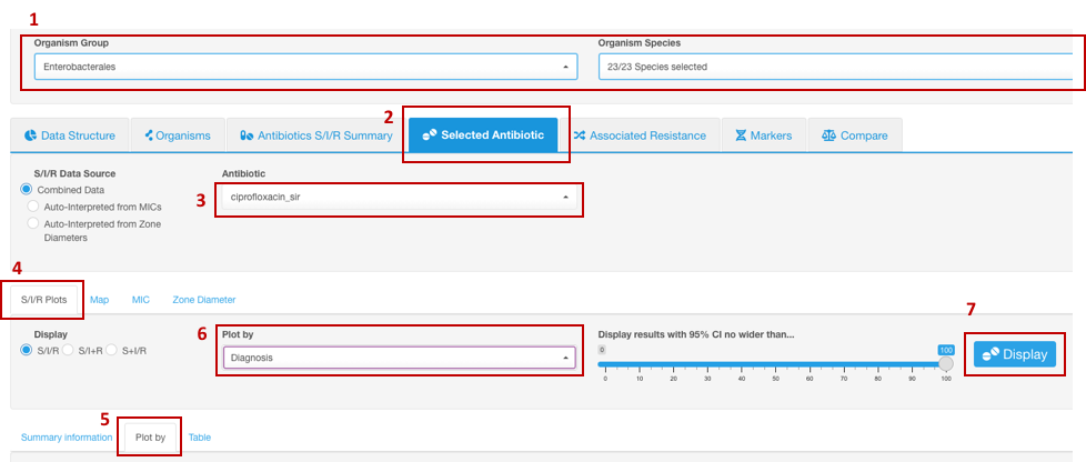
1. Set your Basic Filters to select the Organism Species or Organism Group (e.g., Enterobacterales) that you wish to analyze (Species or group of organisms has to be selected for the tasks involving antimicrobial resistance phenotype interpretation due to the species-specific nature of susceptibility breakpoints).
2. In the Infographics field, select the tab Selected Antibiotic.
3. Under the tab Selected Antibiotic, from the drop-down list, pick the Antibiotic resistance to which you want to explore.
4. Open sub-tab S/I/R Plots.
5. Click on sub-tab Plot by further down.
6. From the appeared drop-down filter Plot by (under S/I/R Plots), chose category Diagnosis (may be named differently depending on the headers title in your dataset).
7. Click the button Display.

Example of data display:

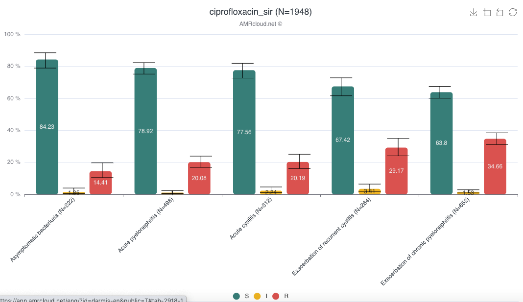
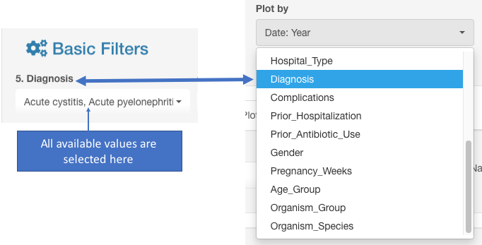
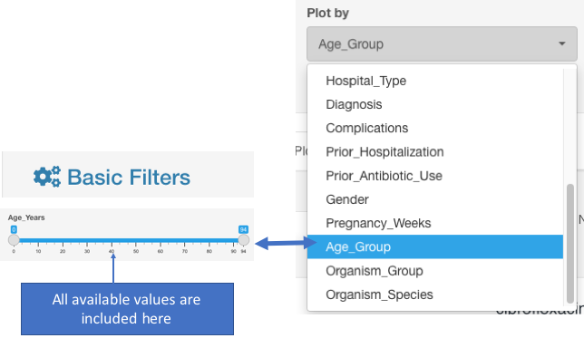
When using the Plot by function, it is important to have all available values selected under Basic Filters for the parameter selected as the category in Plot by. E.g., if Plot by is set to Diagnosis under Selected Antibiotic infographics, the Basic Filter for Diagnosis category should have all values selected:

The analyzed dataset can be further sorted by applying additional Basic Filters. However, after the Basic Filters are modified, the downstream Basic Filters settings will be discarded and would need to be selected again, and the antibiotic name needs to be picked (see chapter Hierarchical sorting principle of this manual for details).

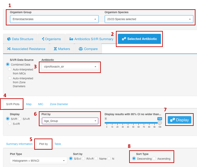
Distribution of resistance in different age groups

1. Set your Basic Filters to select the Organism Species or Organism Group (e.g., Enterobacterales) you wish to analyze. (Species or a group of organisms must be selected for the tasks involving antimicrobial resistance phenotype interpretation due to the species-specific nature of susceptibility breakpoints).
2. In the Infographics field, select the tab Selected Antibiotic.
3. Under the tab Selected Antibiotic, from the drop-down list, pick the Antibiotic resistance to which you want to explore.
4. Open sub-tab S/I/R Plots.
5. Click on sub-tab Plot by further down.
6. From the appeared drop-down filter Plot by (under S/I/R Plots), chose the category Age Group (may be named differently depending on the headers title in your dataset).
7. Click the button Display.
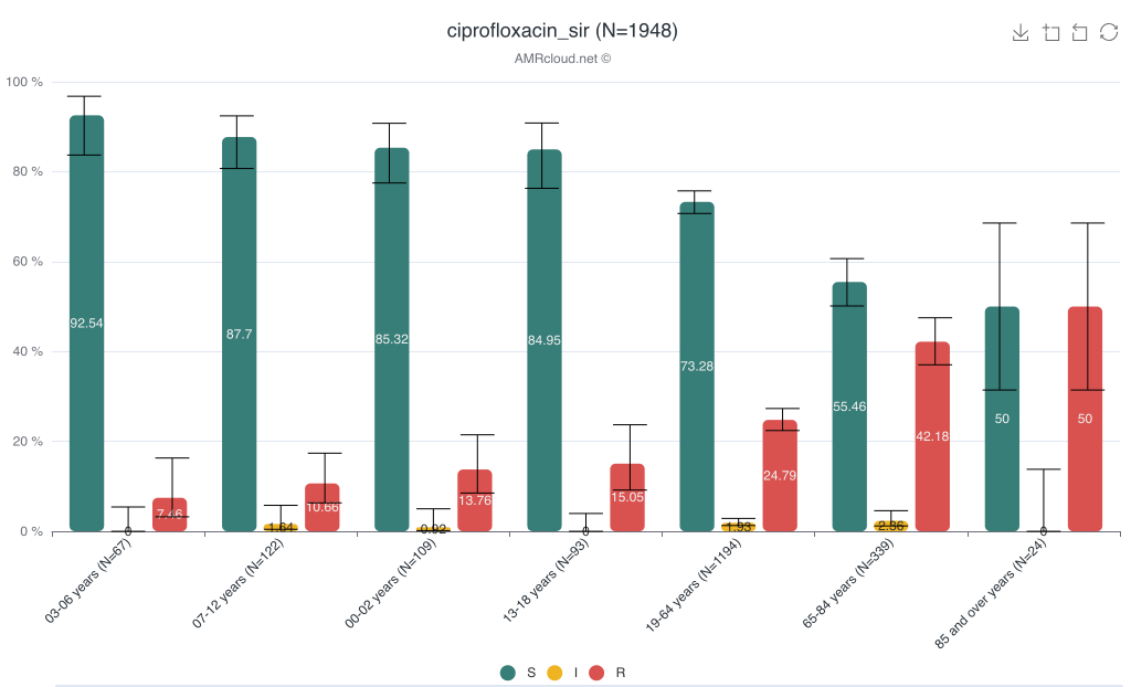
8. To create a graph sorted by age along the X-axis: use graph settings options: Sort By - Name. Sort Type - Descending or Ascending.

Example of data display:

When using Plot by function, it is important to have all available values selected under Basic Filters for the parameter selected as the category in Plot by. E.g., if Plot by is set to Age group under Selected Antibiotic infographics, the Basic Filter for the Age group category should have all values included (unless you intended to exclude them from the analysis):

The analyzed dataset can be further sorted by applying additional Basic Filters. However, after the Basic Filters are modified, the downstream Basic Filters settings will be discarded and would need to be selected again, and the antibiotic name needs to be picked (see chapter Hierarchical sorting principle of this manual for details).

S/I/R distribution for antimicrobials tested within a certain period

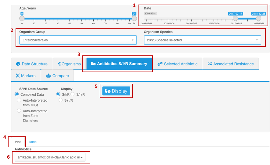
1. Set your Basic Filters to select the date range for the data you wish to include in the analysis.
2. In the Basic Filters, select the Organism Species or Organism Group (e.g., Enterobacterales) that you wish to analyze. (Species or a group of organisms must be selected for the tasks involving antimicrobial resistance phenotype interpretation due to the species-specific nature of susceptibility breakpoints).
3. In the Infographics field, select the tab Antibiotics S/I/R Summary, sub-tab Plot
4. Click the button Display.
5. Under tab Plot, from the drop-down list, pick the Antibiotic resistance to which you want to explore.

Example of data display:

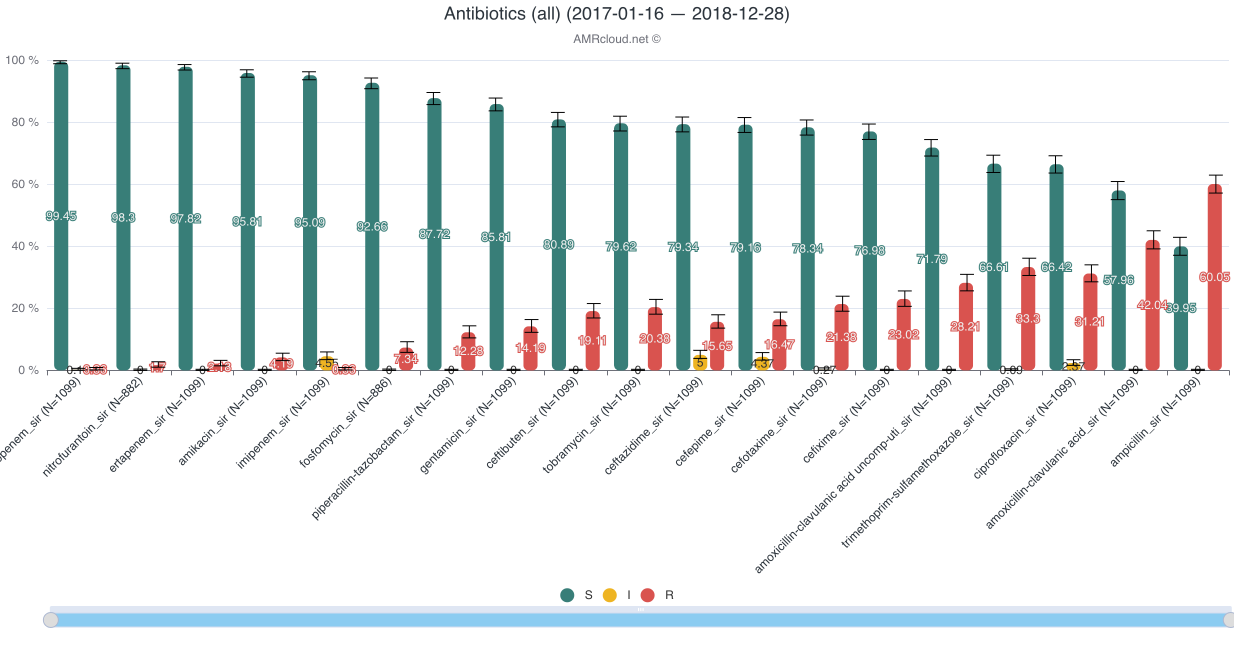
The analyzed dataset can be further sorted by applying additional Basic Filters. However, after the Basic Filters are modified, the downstream Basic Filters settings will be discarded and would need to be selected again, and the antibiotic name needs to be picked (see chapter Hierarchical sorting principle of this manual for details).

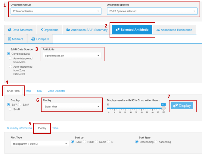
Trends in resistance to an antibiotic over a period of time

1. Set your Basic Filters to select the Organism Species or Organism Group (e.g., Enterobacterales) you wish to analyze. (Species or group of organisms has to be selected for the tasks involving antimicrobial resistance phenotype interpretation due to species-specific nature of susceptibility breakpoints).
2. In the Infographics field, select the tab Selected Antibiotic.
3. Under the tab Selected Antibiotic, from the drop-down list, pick the Antibiotic resistance to which you want to explore.
4. Open sub-tab S/I/R Plots.
5. Click on sub-tab Plot by further down.
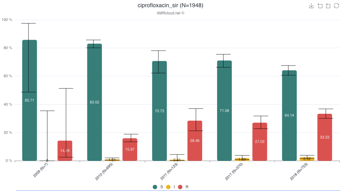
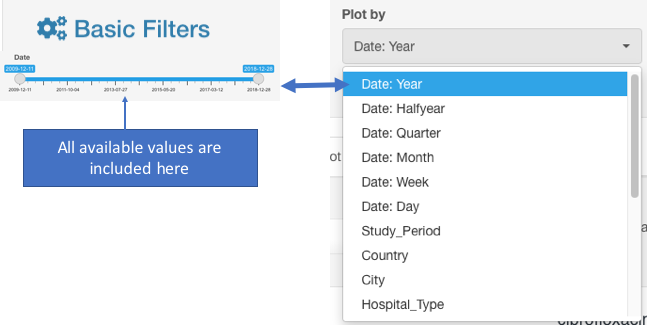
6. From the appeared drop-down filter Plot by (under S/I/R Plots), chose the category Date: Year (may be named differently depending on the header titles in your dataset). AMRcloud algorithm can round the dates to display congregated data by years, quarters, months, and weeks.
7. Click the button Display.
8. Note that dates are always sorted automatically in chronological order, and Descending/Ascending sorting doesn’t work in this infographic.

Example of data display:

Data is presented as histogram by default.

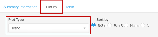
For the presentation of data as resistance trend, under the sub-tab Plot by, select the Trend option from the Plot type drop-down list.

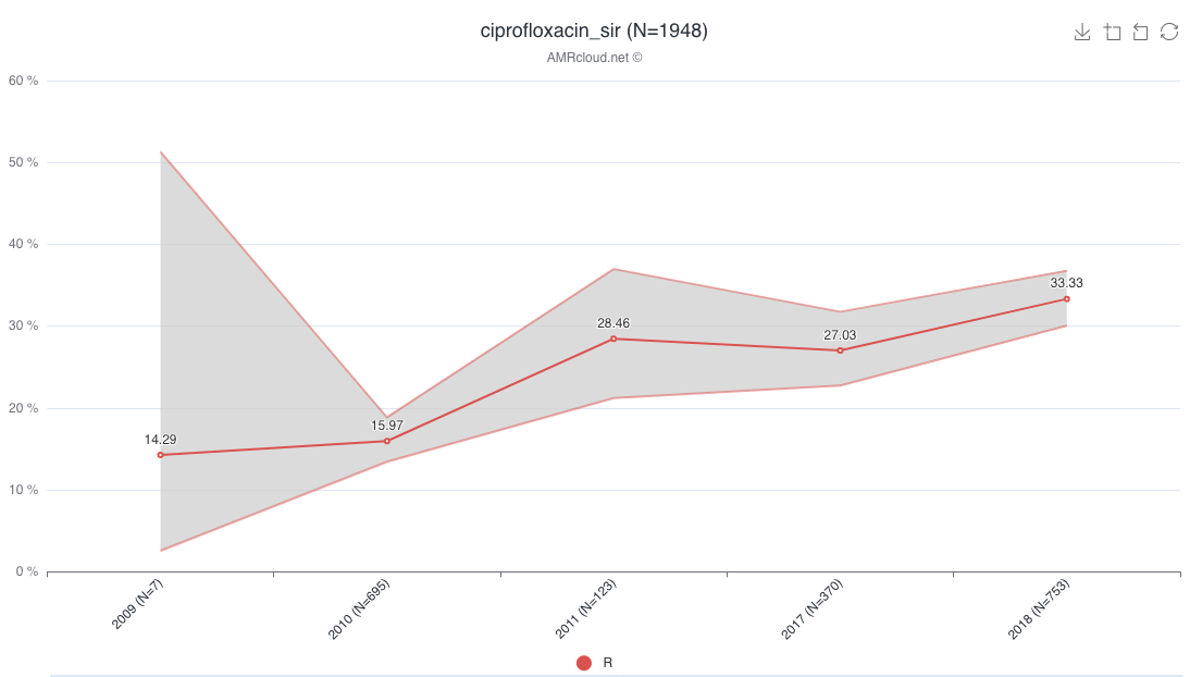
When using Plot by function, it is important to have all available values selected under Basic Filters for the parameter selected as the category in Plot by. E.g., if Plot by is set to Date:Year under Selected Antibiotic infographics, the Basic Filter for the Date category should have all values included (unless you intended to exclude them from the analysis):

The analyzed dataset can be further sorted by applying additional Basic Filters. However, after the Basic Filters are modified, the downstream Basic Filters settings will be discarded and would need to be selected again, and the antibiotic name needs to be picked (see chapter Hierarchical sorting principle of this manual for details).

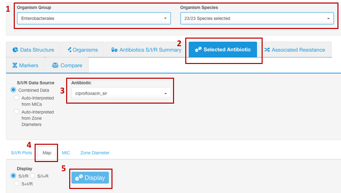
Geographical distribution of resistance profiles (map visualization)

1. Set your Basic Filters to select the Organism Species or Organism Group (e.g., Enterobacterales) you wish to analyze. [Species or a group of organisms must be selected for the tasks involving antimicrobial resistance phenotype interpretation due to the species-specific nature of susceptibility breakpoints].
2. In the Infographics field, select the tab Selected Antibiotic.
3. Under the tab Selected Antibiotic, from the drop-down list, pick the Antibiotic resistance to which you want to explore.
4. Open sub-tab Map.
5. Click the button Display.

View map with overplayed S/I/R data in the infographics “Map” below.

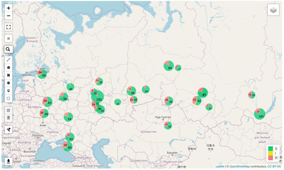
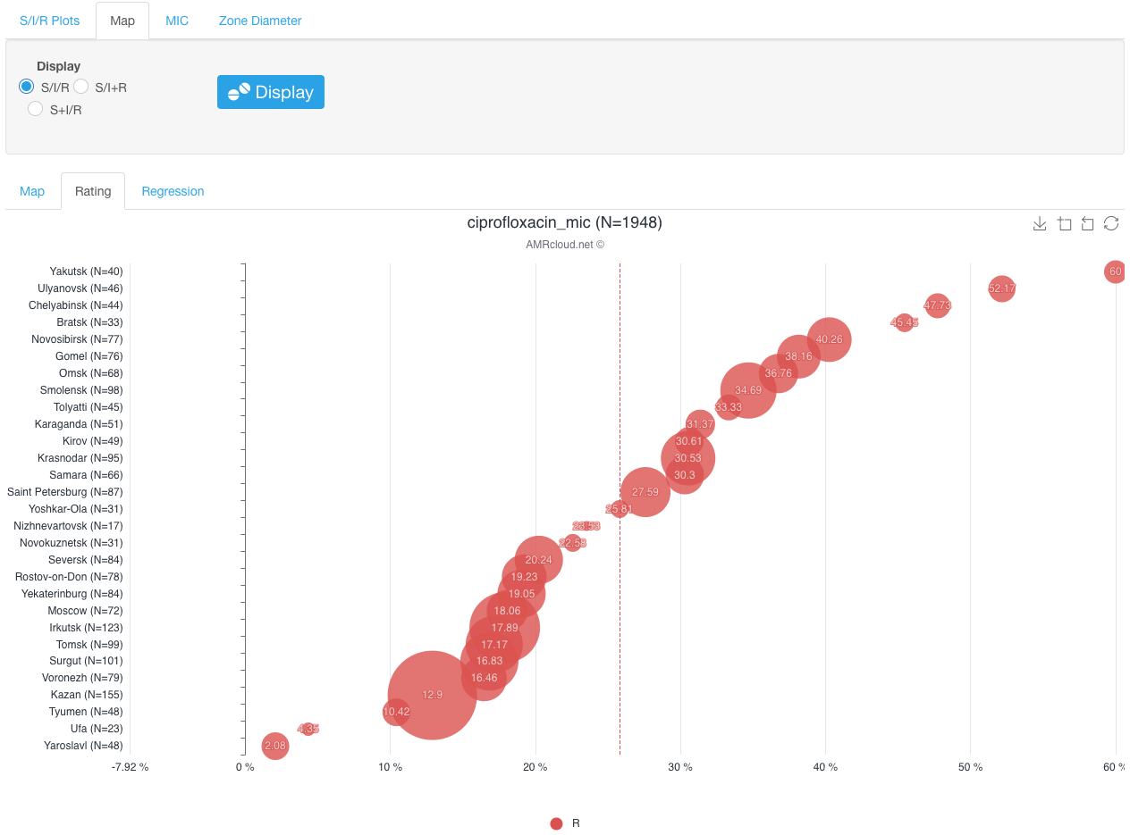
Alternatively, the distribution of relative proportions of isolates resistant to a given antibiotic by geographic locations can be shown by clicking infographics sub-tab Rating (also under Map sub-tab). In the graph below, the prevalence of the selected resistance type in all geographical loci is ordered according to its rate. A vertical dotted line designates a median percentage of resistant isolates.

The analyzed dataset can be further sorted by applying additional Basic Filters. However, after the Basic Filters are modified, the downstream Basic Filters settings will be discarded and would need to be selected again, and the antibiotic name needs to be picked (see chapter Hierarchical sorting principle of this manual for details).

Association of resistance phenotype and genotype

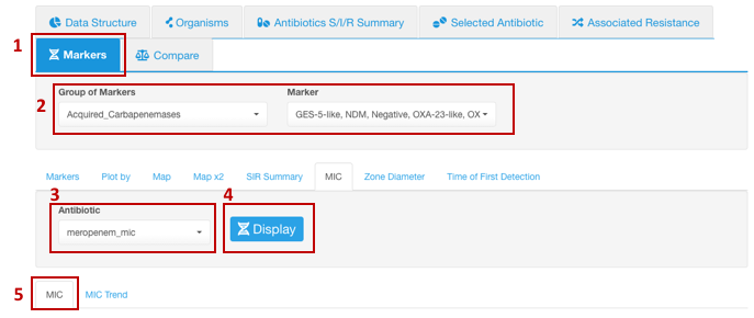
This type of analysis depends on the data uploaded by the user and can be done using the Markers tab. Specifically, it allows to show MIC distribution for the isolates with different genetic resistance determinants present.

1. In the Markers tab, select a group of markers and/or specific markers that you wish to analyze from the corresponding drop-down lists.
2. Select the sub-tab MIC.
3. Select an antibiotic for which you wish to explore the association of phenotype and genotype.
4. Click the button Display.
5. View the histogram of MIC-genetic marker distribution in the infographics MIC below.

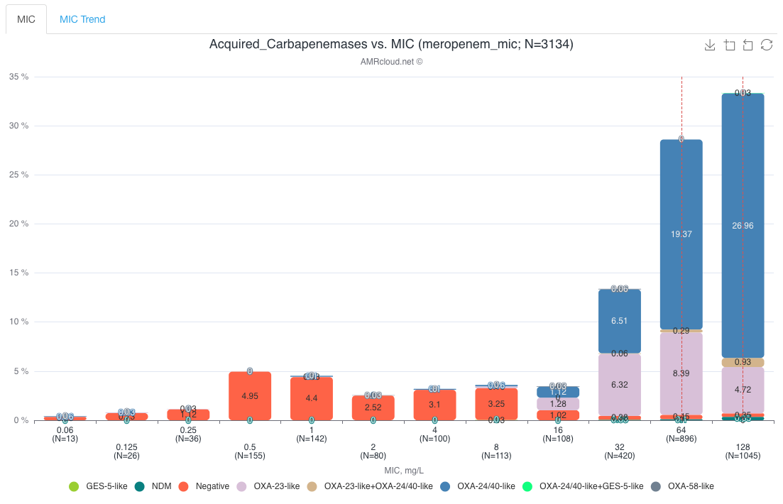
Example of data display. In the provided below example, the presence of carbapenemases correlates with high MIC values of meropenem:

Associated resistance

AMRcloud allows users to explore the association between different antibiotic resistance phenotypes by comparing relative numbers of the isolates resistant to various antibiotics. This information helps to form a better understanding of the general epidemiology of antibiotic resistance and assists with choosing the strategy of antimicrobial prescriptions.

Matrix of associated resistance

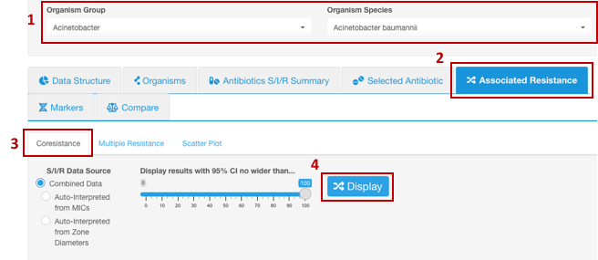
To determine whether any co-resistance is observed in the dataset, use the tab Associated Resistance. A good way to start is with known resistance to an antimicrobial present in your isolates; determine the likelihood of that type of resistance to be associated with the resistance to other antimicrobials. For that:

1. Set your Basic Filters to select the Organism Species or Organism Group (e.g., Enterobacterales) you wish to analyze. (Species or a group of organisms must be selected for the tasks involving antimicrobial resistance phenotype interpretation due to the species-specific nature of susceptibility breakpoints).
2. Under the tab Associated Resistance, select the sub-tab Coresistance.
3. Click the button Display.
4. View the matrix of associated resistance in the infographics Matrix below.

Example of data display:

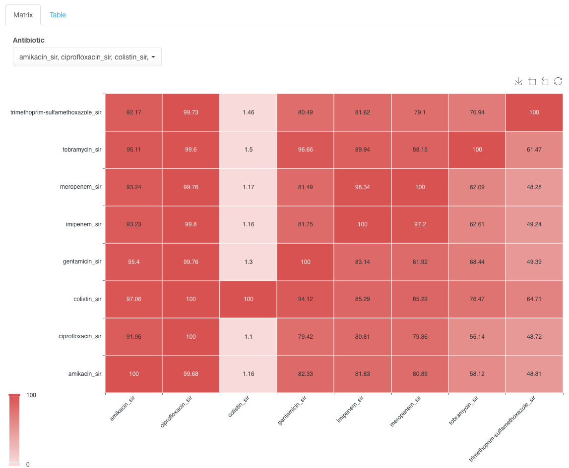
In the example matrix above, find the row with the antibiotic to which the resistance is observed in the dataset and which you want to investigate for co-resistance for other antimicrobials, e.g., meropenem.

Values in the intersections show the likelihood of associated resistance between two drugs being present. E.g., in the example above, there is an 81.49% likelihood that an isolate with resistance to meropenem will also be resistant to gentamicin. Usually, the goal is to find the drug combination with the lowest likelihood value for co-resistance as a potential option for treatment in case of observed resistance to one of the drugs in the pair. Another use of this type of analysis is the detection of unusual resistance patterns, e.g., in the case of resistance of Acetobacter isolates to meropenem, tobramycin has the lowest level of associated resistance among other aminoglycosides.

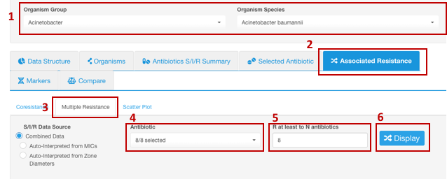
Multiple Resistance

To calculate the proportion of multi-/extreme-/pan-drug-resistant isolates (as determined by the user) in your dataset, use sub-tab Multiple Resistance. This function allows the user to determine the percentage of isolates that are resistant to at least one, two, … N number of antibiotics simultaneously. The user can specify antimicrobials selected for the analysis.

1. Set your Basic Filters to select the Organism Species or Organism Group (e.g., Enterobacterales) you wish to analyze.
2. Select the tab Associated Resistance,
3. Select the sub-tab Multiple Resistance.
4. Pick the antibiotics, among which multiple resistance will be explored. Multiple resistance will only be analyzed among the selected antibiotics (selecting only one antibiotic will not allow analyzing for multiple resistance).
5. Enter the number of antimicrobials to which the simultaneous resistance must be observed in your selected group (user defines the multiple resistance in this analysis). E.g., in the example below, to determine the proportion of isolates that are resistant to all antibiotics in the panel (pan-resistance), select all antibiotics in the dataset (8 out of 8) in the field Antibiotic and set N number to 8 in the field R at least to N antibiotics.
6. Click the button Display.

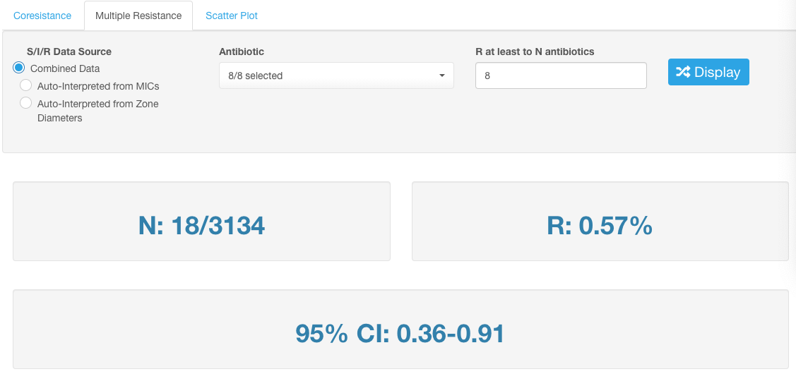
View the number of isolates meeting the set parameters of multiple resistance. The percentage value from the total number of isolates in the dataset and 95% confidence interval (CI) are also calculated automatically.

The analyzed dataset can be further sorted by applying additional Basic Filters. However, after the Basic Filters are modified, the downstream Basic Filters settings will be discarded and would need to be selected again, and the antibiotic name needs to be picked (see chapter Hierarchical sorting principle of this manual for details).

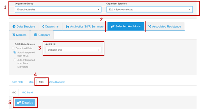
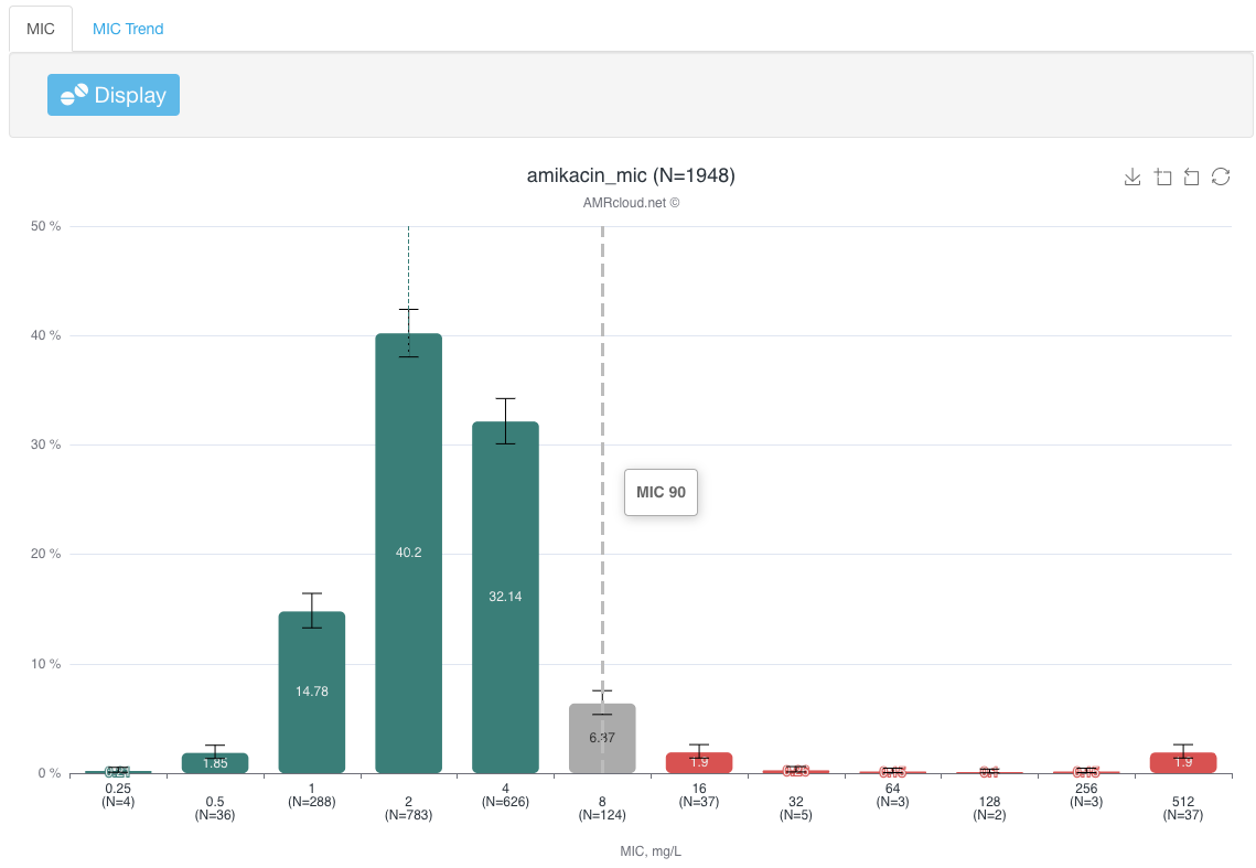
Visualize MIC 50 and MIC 90

1. Set your Basic Filters to select the Organism Species or Organism Group (e.g., Enterobacterales) you wish to analyze. (Species or a group of organisms must be selected for the tasks involving antimicrobial resistance phenotype interpretation due to the species-specific nature of susceptibility breakpoints).
2. In the Infographics field, select the tab Selected Antibiotic.
3. Under the tab Selected Antibiotic, from the drop-down list, pick the Antibiotic resistance to which you want to explore.
4. Open sub-tab MIC.
5. Click the button Display.

In the infographics MIC below, the MIC50 and MIC90 will be displayed as dotted vertical lines above corresponding MIC columns. Hovering over the dotted line will bring out the corresponding MIC50 or MIC90 label:

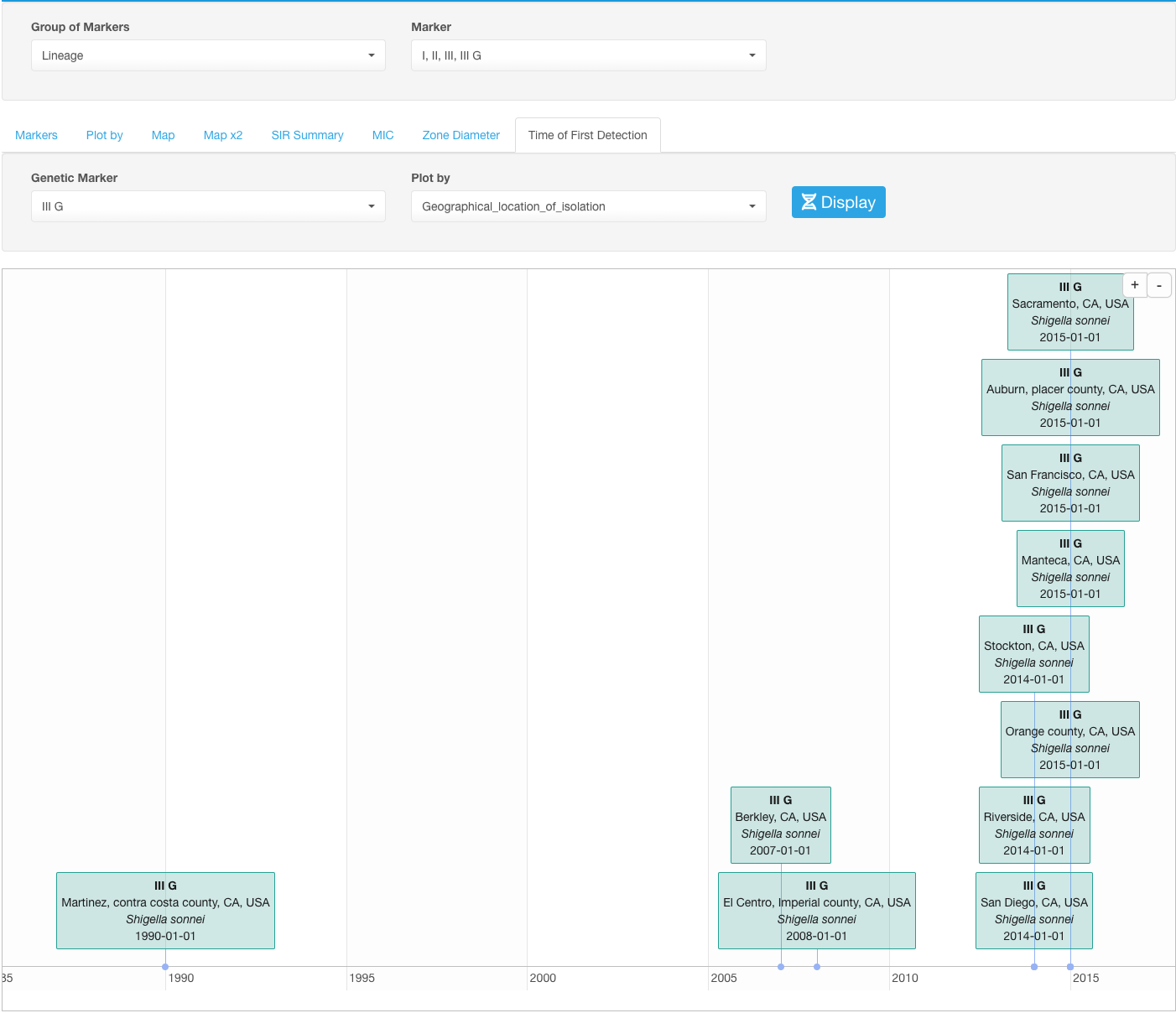
Time of First Detection of a certain marker in different geographical locations

It could be useful to visualize the timeline of occurrence of certain markers- virulence or resistance determinant or a genetic lineage- in different geographical locations available in your dataset. For that, perform the following steps:

1. Set your basic filters to include/filter data that you would like to analyze.
2. In the Infographics field, select the tab Markers.
3. Under the Markers tab, chose the group of markers you would like to analyze in the Group of Markers drop-down list. You don’t have to select a specific Marker at this level because you will be selecting the specific marker for visualization later.
4. Open sub-tab Time of First Detection.
5. Select the marker under the drop-down list Genetic Marker.
6. Select the geographical location parameter under Plot by drop-down list.
7. Click the button Display.

For example: if we select an IIIG lineage of Shigella sonnei in our example dataset as a Genetic Marker and set the Plot by to the geographical location of isolation, we will see the dates when IIIG lineage was first isolated in different geographical locations: